Indexing data to a common starting point
The economic problem
Indexing is kind of like a race
That a racehorse can run is relatively uninteresting. Of more intrigue to bookies and bettors is that a given racehorse can run relatively faster than another. Few would come to watch randomly placed horses gallop around a track, each starting and stopping at will and each with its own finish line. It’s the comparison of competing horses and subsequent ranking that make a race compelling.
To create a fair comparison, track officials normalize the beginning point with a start gate, release all horses at the same time and use precision measuring instruments to determine a winner. Clearly, some racehorses are faster and stronger than others. But without a common starting point, any determination of physical supremacy would be dubious.
A similar case holds true with economic data. Economists like to compare data. They do so to gain perspective and to put things in context. For instance, knowing that a state’s employment is growing over time is useful. But knowing its growth rate relative to other states is more telling. For example, a state’s rate of employment change, though positive, could be the weakest of the 50 states in a sample.
Start data at the same point
A relatively simple way to make such comparisons is by indexing data to a common starting point. In effect, the variables in question must be set equal to each other and then examined over time for differences. Indexed data are handy because they allow an observer to quickly determine rates of growth by looking at a chart’s vertical axis. They also allow for comparison of variables with different magnitudes.
Indexing enables comparison of data of any magnitude
For example, suppose an analyst wants to use a graph to compare the gross domestic product (GDP) of three different countries. Drawing such a chart with absolute values would be difficult because of the size disparity between countries. One country’s GDP might register in the trillions, another in the hundreds of billions and the other in the tens of billions. All these amounts wouldn’t fit well on the chart.
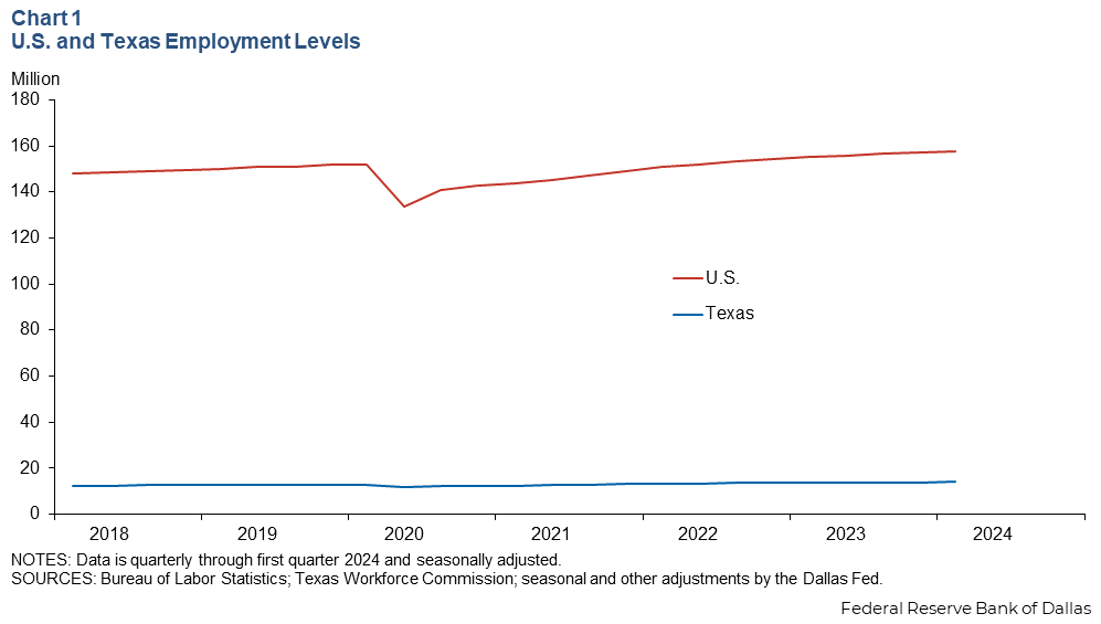
Take as another example, an analyst wants to determine whether the U.S. or Texas recovered lost jobs from the COVID-19 pandemic more quickly. Chart 1 shows how dissimilar magnitudes in employment levels in Texas and the United States make for difficult graphical interpretation. This chart demonstrates that the level of employment in the U.S. is substantially larger than employment in Texas, but because of this large disparity in magnitude, it’s impossible to tell from this chart whether employment recovered in Texas faster or slower than the U.S.
Indexing numerical data is useful in a variety of contexts. It shows up all the time in economic, financial and business analysis. Equity traders index stock prices and stock indices to compare performance over time. Economists index data to prominent events—say economic peaks (or troughs)—to see how the data decline (or rise) relative to each other. In all cases, it allows for quick comparison and ranking.
The technical solution
Indexing mechanics
To index numerical data, values must be adjusted so they are equal to each other in a given starting time period. By convention, this value is usually 100. From there on, every value is normalized to the start value, maintaining the same percentage changes as in the nonindexed series. Subsequent values are calculated so that percent changes in the indexed series are the same as in the nonindexed.
Consider the data in Table 1. Variables X and Y represent hypothetical data series. On average variable Y is one order of magnitude larger than variable X. To index the two series, apply the following equation to the raw data:
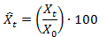
Where Xt is the raw data value in a given time period from t = 2011, 2012…2024, X0 is the data value in the initial time period, 2011 and X^t is the new indexed value of the variable.
| Table 1 Indexing two data series |
||||
| Year | X | Y | Indexed value of X |
Indexed value of Y |
| 2011 | 250 | 2,000 | 100 | 100 |
| 2012 | 500 | 3,000 | 200 | 150 |
| 2013 | 810 | 6,000 | 324 | 300 |
| 2014 | 925 | 6,500 | 370 | 325 |
| 2015 | 1,010 | 6,500 | 404 | 325 |
| 2016 | 1,052 | 7,100 | 421 | 355 |
| 2017 | 1,030 | 7,300 | 412 | 365 |
| 2018 | 1,240 | 7,600 | 496 | 380 |
| 2019 | 1,470 | 7,800 | 588 | 390 |
| 2020 | 1,500 | 8,300 | 600 | 415 |
| 2021 | 1,525 | 9,200 | 610 | 460 |
| 2022 | 1,580 | 9,900 | 632 | 495 |
| 2023 | 1,740 | 10,200 | 696 | 510 |
| 2024 | 1,890 | 9,800 | 756 | 490 |
Between 2011 and 2012, variable X increased from 250 to 500, or 100 percent. Consequently, the indexed value of X must also increase 100 percent, from 100 to 200. Similarly, Y increased 50 percent between 2011 and 2012. Thus the indexed value of Y increased 50 percent, from 100 to 150, over the same time period.
Indexing allows you to quickly gauge percentage changes between the initial time period and any subsequent time period. For example, between 2011 and 2024, variables X and Y increased 656 and 390 percent, respectively.
Real-world example
Applying the technique to Texas and U.S. employment
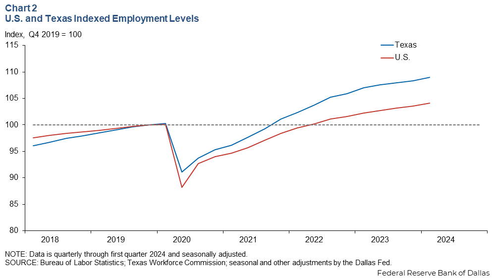
Indexing improves the ability to analyze changes in data over a specified time period. In the example of the U.S. and Texas employment levels, it was difficult to see how job growth in Texas compared with job growth at the national level. However, such a comparison is possible with indexed data.
The calculations
In Table 2 to index data to fourth quarter 2019, each value in the U.S. column is divided by 151,638 and multiplied by 100 to arrive at an indexed value. Likewise, each value in the Texas column is divided by 12,905 and multiplied by 100.
| Table 2 Indexing Texas and U.S. employment data |
||||
| Period | U.S. | Texas | U.S. indexed | Texas indexed |
| Q1 2018 | 148,000 | 12,394 | 97.6 | 96.0 |
| Q2 2018 | 148,716 | 12,486 | 98.1 | 96.8 |
| Q3 2018 | 149,219 | 12,573 | 98.4 | 97.4 |
| Q4 2018 | 149,650 | 12,635 | 98.7 | 97.9 |
| Q1 2019 | 150,141 | 12,706 | 99.0 | 98.5 |
| Q2 2019 | 150,695 | 12,779 | 99.4 | 99.0 |
| Q3 2019 | 151,149 | 12,859 | 99.7 | 99.6 |
| Q4 2019 | 151,638 | 12,905 | 100.0 | 100.0 |
| Q1 2020 | 151,750 | 12,947 | 100.1 | 100.3 |
| Q2 2020 | 133,705 | 11,762 | 88.2 | 91.1 |
| Q3 2020 | 140,611 | 12,096 | 92.7 | 93.7 |
| Q4 2020 | 142,590 | 12,303 | 94.0 | 95.3 |
| Q1 2021 | 143,544 | 12,413 | 94.7 | 96.2 |
| Q2 2021 | 145,153 | 12,606 | 95.7 | 97.7 |
| Q3 2021 | 147,231 | 12,813 | 97.1 | 99.3 |
| Q4 2021 | 149,175 | 13,052 | 98.4 | 101.1 |
| Q1 2022 | 150,753 | 13,206 | 99.4 | 102.3 |
| Q2 2022 | 151,972 | 13,393 | 100.2 | 103.8 |
| Q3 2022 | 153,285 | 13,577 | 101.1 | 105.2 |
| Q4 2022 | 154,114 | 13,672 | 101.6 | 105.9 |
| Q1 2023 | 155,013 | 13,816 | 102.2 | 107.1 |
| Q2 2023 | 155,766 | 13,886 | 102.7 | 107.6 |
| Q3 2023 | 156,433 | 13,928 | 103.2 | 107.9 |
| Q4 2023 | 157,050 | 13,983 | 103.6 | 108.4 |
| Q1 2024 | 157,822 | 14,065 | 104.1 | 109.0 |
Texas grew faster than the U.S. over the study period
Chart 2 illustrates the effect of indexing the two data series. At the onset of the pandemic in March 2020, Texas lost comparatively fewer jobs than the U.S. In addition, its recovery has been faster—reaching pre-pandemic levels of employment in 2021, whereas the U.S. recovered to that amount only in 2022.
Summary
The indexing methodology can be used with various types of economic data. It can be an effective means of normalizing data to a common starting point and observing how variables change over time relative to each other. It is a common method used by economists and businesspeople to enhance perspective and understanding of economic trends.
Glossary at a glance
- Indexing:
- Modifying two or more numeric data series so that the resulting series start at the same value and change at the same rate as the unmodified series.