Smoothing data with moving averages
The economic problem
Economists use smoothing techniques to help show the economic trend in data
To decipher trends in data series, researchers perform various statistical manipulations. These operations are referred to as “smoothing techniques” and are designed to reduce or eliminate short-term volatility in data. A smoothed series is preferred to a non-smoothed one because it may capture changes in the direction of the economy better than the unadjusted series does.
Seasonal adjustment is one smoothing technique
One common smoothing technique used in economic research is seasonal adjustment. This process involves separating out fluctuations in the data that recur in the same month every year (seasonal factors). Such fluctuations can be a result of annual holidays (a jump in December retail sales) or predictable weather patterns (an increase in homebuilding in the spring). For further information on the seasonal adjustment process, see “Seasonally Adjusting Data.”
A moving average can smooth data that remains volatile after seasonal adjustment
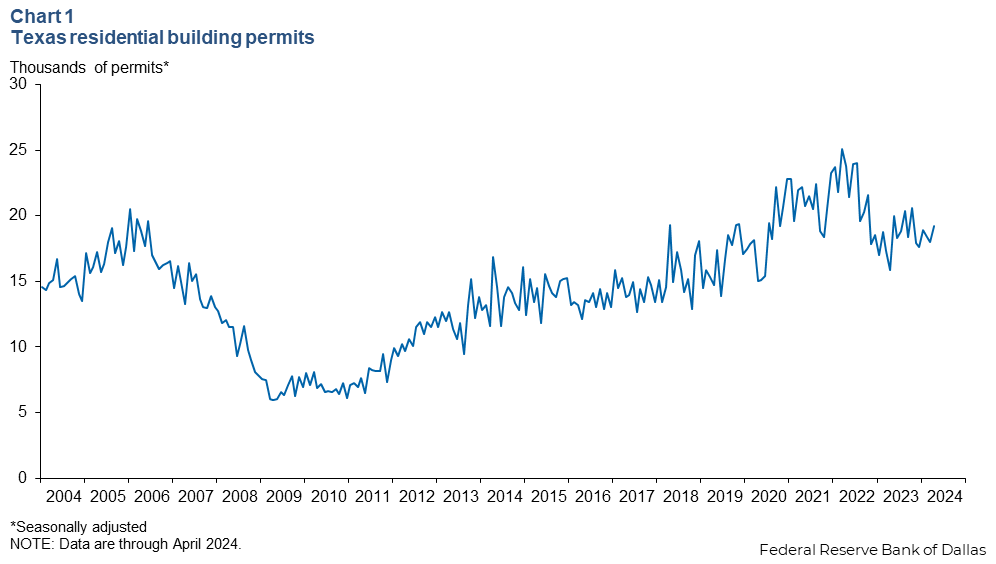
In other cases, a data series retains volatility even after seasonal adjustment. A good example is housing permits, which exhibit strong seasonal fluctuations primarily due to predictable weather patterns. Even after seasonal adjustment eliminates these predictable patterns, however, considerable volatility remains (Chart 1). Why? Because seasonal adjustment does not account for irregular factors such as unusual weather conditions or natural disasters, among others. Such events are unexpected and cannot be isolated the way seasonal factors can. For instance, did single-family housing permits fall in June because economic conditions worsened, or was it just a wetter June than usual? Economists use a simple smoothing technique called “moving average” to help determine the underlying trend in housing permits and other volatile data. A moving average smoothes a series by consolidating the monthly data points into longer units of time—namely an average of several months’ data.
There is a downside to using a moving average to smooth a data series, however. Because the calculation relies on historical data, some of the variable’s timeliness is lost. For this reason, some researchers use a “weighted” moving average, where the more current values of the variable are given more importance. Another way to reduce the reliance on past values is to calculate a “centered” moving average, where the current value is the middle value in a five-month average, with two lags and two leads. The lead figures are forecasted values. Data available from the Dallas Fed’s web site are adjusted using the simple moving average technique explained below.
The technical solution
The formula for a simple moving average is:
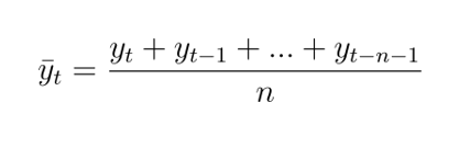
where y is the variable (such as single-family housing permits), t is the current time period (such as the current month), and n is the number of time periods in the average. In most cases, researchers use three-, four- or five-month moving averages (so that n = 3, 4 or 5), with the larger the n, the smoother the series.
Real-world example
Texas housing permits are volatile from month to month; a moving average helps show the underlying trend in the data
| Table 1 | ||
| Month | Single-family housing permits (seasonally adjusted) |
Five-month moving average, single-family housing permits (seasonally adjusted) |
| April 2023 | 15,840 | 17,497 |
| May 2023 | 19,960 | 17,777 |
| June 2023 | 18,312 | 18,038 |
| July 2023 | 18,865 | 18,057 |
| August 2023 | 20,386 | 18673 |
| September 2023 | 18,410 | 19,187 |
| October 2023 | 20,577 | 19,310 |
| November 2023 | 17,918 | 19,231 |
| October 2023 | 20,577 | 19,310 |
| November 2023 | 17,918 | 19,231 |
| December 2023 | 17,623 | 18,983 |
| January 2024 | 18,900 | 18,686 |
| February 2024 | 18,397 | 18,683 |
| March 2024 | 18,000 | 18,168 |
| April 2024 | 19,237 | 18,431 |
In the third column, the bottom figure (18,431) is found by taking the average of the current month and the previous four months in column two.

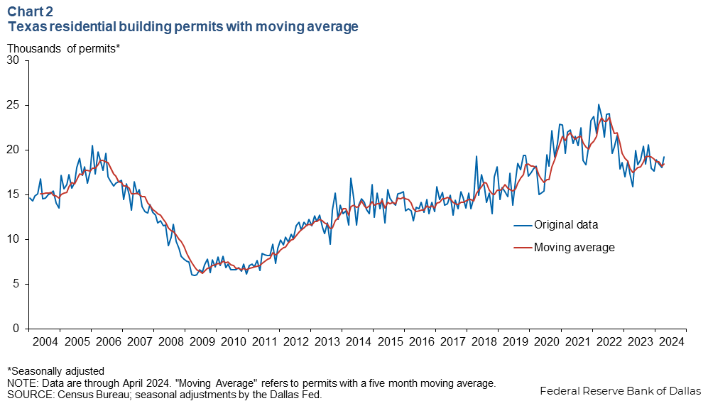
The series in the third column is smoothed, and as Chart 2 shows, is much less volatile than the original series. Using the smoothed data, a researcher can more easily determine underlying trends in the data, as well as detect significant changes in direction.
Summary
Smoothing techniques reduce the volatility in a data series, which allows analysts to identify important economic trends. The moving average technique offers a simple way to smooth data; however, because it utilizes data from past time periods, it may obscure the latest changes in the trend.
Glossary at a glance
- Moving average:
- A calculation that smoothes a volatile data series by averaging neighboring data points.
- Seasonal adjustment:
- The type of smoothing technique in which seasonal fluctuations in the data are estimated and removed.
- Smoothing technique:
- A statistical operation performed on economic data series to reduce or eliminate short-term volatility.