Deflating nominal values to real values
The economic problem
Importance of tracking economic data
Business and economic researchers like to tally things. They count everything from jobs and houses to cars and toasters. In the aggregate, such information is important because it helps show at what rate the economy is expanding or contracting. And the rate at which the economy grows (independent of population growth) plays an integral part in overall economic well-being.
But some economic concepts are difficult to measure
Even though measuring any part of the economy creates certain logistical challenges, some concepts are simply harder to quantify than others. For example, keeping track of a meaningful measure of retail sales over a 10-year period presents more difficulty than simply recording housing starts in a given neighborhood.
So count dollar value, not quantity
Enumerating housing starts is straightforward. Measuring retail sales, on the other hand, is not so easy. Retail goods comprise any number of different products, ranging from computers, kitchen appliances and clothing to auto parts and garden tools. This characteristic of the variable complicates the counting. Statistics keepers avoid the problem by tracking retail sales by dollar amounts, not quantity.
But price fluctuations distort the data
However, tracking data in this way presents another problem. Since retail sales are measured in dollars, changes in price levels over time tend to distort reported figures. In the case of retail transactions, economists are interested in tracking actual sales, independent of any price movements. This enables them to make sensible comparisons across time periods even as prices move. Unadjusted for, price fluctuations distort the measurement of economic variables measured in dollar values.
$1 doesn’t buy what it used to
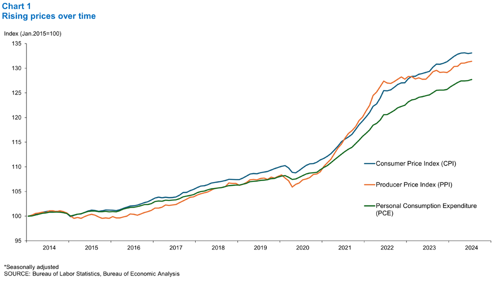
While there’s still debate over which measure of overall price fluctuation is best, the phenomenon of general price movements over time—either deflation or inflation—is undisputed (Chart 1). A few anecdotes help make the point. Some folks can still remember five-cent candy bars and 29-cent gasoline. It hasn’t been too long since hamburger sold at three pounds for a dollar and chicken went for 29 cents a pound. The same four-bedroom house that changed hands for $23,500 in 1970 could easily sell for over $250,000 today.

Solution: remove price effects from the data
In effect, $20 will buy less retail output today than it did 20 years ago. But for data collectors, a $20 purchase gets added to total sales in the same manner today as it did 20 years ago, even though it represents a different quantity of goods. Separating out the price effect leaves researchers with a clearer picture of what’s really happening to sales levels relative to any time period. The object then becomes to remove any part of the variable’s change that is attributable to price movements, arriving at a real, or inflation adjusted, indicator.
The technical solution
Lesser known data unadjusted for inflation
Though many prominent economic series such as gross domestic product (GDP) and exports are adjusted for inflation, some less prominent indicators are not. A simple methodology can be used to deflate any nominal data series to real values.
Changing nominal to real
To transform a series into real terms, two things are needed: the nominal data and an appropriate price index. The nominal data series is simply the data measured in current dollars and gathered by a government or private survey. The appropriate price index can come from any number of sources. Among the more prominent price indexes are the Consumer Price Index (CPI), the Producer Price Index (PPI), the Personal Consumption Expenditure index (PCE) and the GDP deflator.
Common price indexes measure the value of a basket of goods in a certain time period, relative to the value of the same basket in a base period. They are calculated by dividing the value of the basket of goods in the year of interest by the value in the base year. By convention, this ratio is then multiplied by 100.
Generally speaking, statisticians set price indexes equal to 100 in a given base year for convenience and reference. To use a price index to deflate a nominal series, the index must be divided by 100 (decimal form). The formula for obtaining a real series is given by dividing nominal values by the price index (decimal form) for that same time period:

Mechanics of price-level effects on economic data
But how does this simple formula remove price fluctuations from actual changes in a variable’s overall value? Economic variables measured in dollar values like GDP, exports, construction contract values, venture capital and retail sales are calculated from the product of the quantity sold and the selling price. Analysts want to get their hands around the changes in quantity sold and disregard changes in prices because it’s the quantity of goods and services consumed by households that affects well-being, not the prices. In effect, the percentage change in real values over a given time period should mirror the percentage change in quantity.
Three sample scenarios
Table 1 provides three scenarios that show how to correct the data for price fluctuations.
In each scenario price and quantity are multiplied together to arrive at a nominal value in 2015 and 2020. Then the 2020 nominal value is divided by the ratio of the 2020 price index and the 2015 price index to arrive at a real value (or the 2020 value in 2015 dollars).
| Table 1 Deflating 2010 values to 2005 dollars |
||||||
| Scenario | Period | Price | Quantity | Nominal value | Deflating nominal to real | Real value |
| 1. Price rises 50%, quantity stays same | 2015 | 100 | 12 | 1,200 | 1,200 | |
| 2020 | 150 | 12 | 1,800 | 1,800/ (150/100) = |
1,200 | |
| 2. Price stays the same, quantity rises 50% | 2015 | 100 | 12 | 1,200 | 1,200 | |
| 2020 | 100 | 18 | 1,800 | 1,800/ (100/100) = |
1,800 | |
| 3. Price rises 20%, quantity rises 25% | 2015 | 100 | 12 | 1,200 | 1,200 | |
| 2020 | 120 | 15 | 1,800 | 1,800/ (120/100) = |
1,500 | |
The mechanics of each scenario
-
Scenario 1
Prices rise 50 percent from 2015 to 2020 but the quantity stays the same.
Result: The nominal value increases 50 percent, but the real value remains the same.
-
Scenario 2
The price remains constant but quantity increases by 50 percent.
Result: The real value rises by 50 percent.
-
Scenario 3
The price rises 20 percent and quantity rises 25 percent.
Result: After deflating the 2020 value to 2015 dollars, the real value rises 25 percent.
Real-world example
Texas housing permits are volatile from month to month; a moving average helps show the underlying trend in the data
Finally, a real-world example is in order. Table 2 shows how to deflate four-and-a-half years of nominal quarterly GDP data to real GDP. Column 2 shows nominal GDP. Column 3 is the price series. Column 4 reindexes the price series to the first quarter of 2015 by dividing all price values by 236.2 and multiplying by 100. Column 5 puts the price index in decimal form. Column 6 divides nominal GDP by the price index in decimal form to arrive at real GDP—or GDP not affected by price volatility.
| Table 2 Deflating nominal Texas GDP |
|||||
| Period | Nominal GDP (millions of dollars) |
CPI price index |
Reindex to 2015 (Q1 2015=100) | Decimal |
Real GDP (2015 dollars) |
| 2015 - Q1 | 1,577 | 236.2 | 100.0 | 1.000 | 1,577 |
| 2015 - Q2 | 1,580 | 237.6 | 100.6 | 1.006 | 1,571 |
| 2015 - Q3 | 1,590 | 237.4 | 100.5 | 1.005 | 1,581 |
| 2015 - Q4 | 1,592 | 238.1 | 100.8 | 1.008 | 1,579 |
| 2016 - Q1 | 1,571 | 238.2 | 103.1 | 1.031 | 1,558 |
| 2016 - Q2 | 1,595 | 240.0 | 101.6 | 1.016 | 1,570 |
| 2016 - Q3 | 1,607 | 240.9 | 102.0 | 1.020 | 1,575 |
| 2016 - Q4 | 1,608 | 242.9 | 102.8 | 1.028 | 1,564 |
| 2017 - Q1 | 1,625 | 243.9 | 103.3 | 1.033 | 1,573 |
| 2017 - Q2 | 1,632 | 243.9 | 103.3 | 1.033 | 1,580 |
| 2017 - Q3 | 1,640 | 246.4 | 104.3 | 1.043 | 1,571 |
| 2017 - Q4 | 1,676 | 247.9 | 105.0 | 1.050 | 1,597 |
| 2018 - Q1 | 1,724 | 249.6 | 105.7 | 1.057 | 1,631 |
| 2018 - Q2 | 1,744 | 251.0 | 106.3 | 1.063 | 1,641 |
| 2018 - Q3 | 1,762 | 252.1 | 106.7 | 1.067 | 1,651 |
| 2018 - Q4 | 1,773 | 252.6 | 107.0 | 1.070 | 1,657 |
| 2019 - Q1 | 1,772 | 254.2 | 107.7 | 1.077 | 1,646 |
| 2019 - Q2 | 1,784 | 255.0 | 108.0 | 1.080 | 1,652 |
| 2019 - Q3 | 1,813 | 256.4 | 108.6 | 1.086 | 1,670 |
| 2019 - Q4 | 1,832 | 258.4 | 109.4 | 1.094 | 1,674 |
| 2020 - Q1 | 1,802 | 258.1 | 109.3 | 1.093 | 1,649 |
| 2020 - Q2 | 1,678 | 256.6 | 108.6 | 1.086 | 1,545 |
| 2020 - Q3 | 1,798 | 260.0 | 110.1 | 1.101 | 1,633 |
| 2020 - Q4 | 1,814 | 262.1 | 111.0 | 1.110 | 1,634 |
| 2021 - Q1 | 1,846 | 264.8 | 112.1 | 1.121 | 1,646 |
| 2021 - Q2 | 1,895 | 270.3 | 114.4 | 1.144 | 1,656 |
| 2021 - Q3 | 1,916 | 274.0 | 116.0 | 1.160 | 1,651 |
| 2021 - Q4 | 1,946 | 280.7 | 118.9 | 1.189 | 1,637 |
| 2022 - Q1 | 1,955 | 287.4 | 121.7 | 1.217 | 1,606 |
| 2022 - Q2 | 1,955 | 294.7 | 124.8 | 1.248 | 1,567 |
| 2022 - Q3 | 1,979 | 296.4 | 125.5 | 1.255 | 1,576 |
| 2022 - Q4 | 2,010 | 299 | 126.6 | 1.266 | 1,588 |
| 2023 - Q1 | 2,033 | 301.6 | 127.7 | 1.277 | 1,592 |
| 2023 - Q2 | 2,049 | 303.4 | 128.5 | 1.285 | 1,595 |
| 2023 - Q3 | 2,085 | 307.4 | 130.2 | 1.302 | 1,602 |
| 2023 - Q4 | 2.111 | 309.2 | 130.9 | 1.309 | 1,612 |
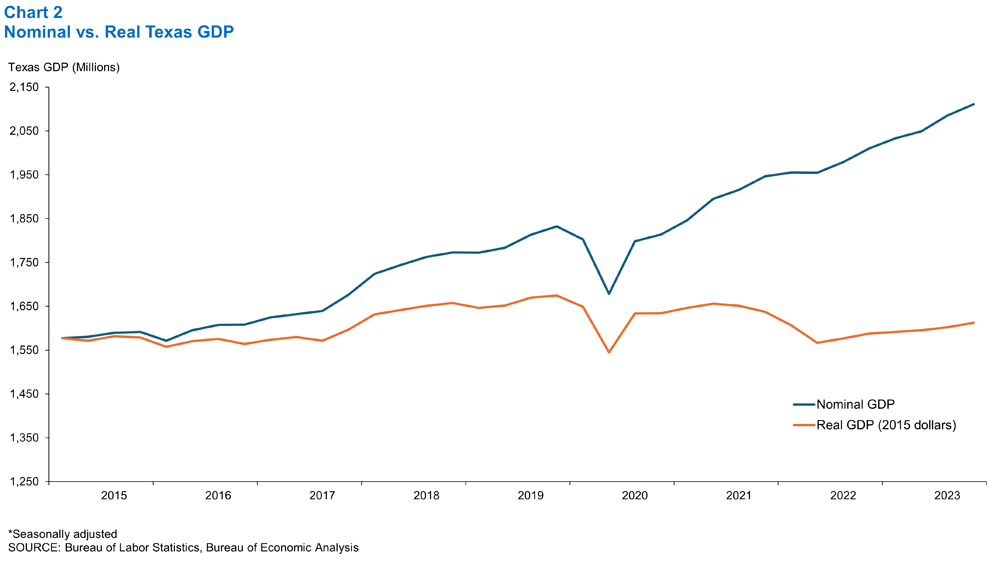
Chart 2 illustrates the point graphically. As expected, nominal GDP grows faster than real GDP because it includes inflation. Real GDP growth appears more moderate because the calculation has separated out any pricing effects. The real measure is a better overall indication of the change in output over the sample time period.

Summary
Increases in nominal values, such as the total dollars of retail sales, may arise from increases in prices or increases in quantities sold. Only an increase in quantity points to an improvement in economic well-being, so analysts need an effective way to determine the importance of these competing explanations. Converting nominal values to real values provides a consistent measure across time.
Glossary at a glance
- Deflator:
- A numeric pricing measure used to change nominal values into real values.
- Homogeneous:
- Of the same or a similar kind or nature.
- Nominal:
- The value of an economic variable in terms of the price level at the time of its measurement; or, unadjusted for price movements.
- Real:
- The value of an economic variable adjusted for price movements.