Productivity the key to raising living standards

There has been incredible stability in the rate of improvement in U.S. living standards over time. As first documented by Stanford economist Charles Jones, living standards, measured by GDP per capita, have risen at a pretty constant rate of 1.9 percent per year in the U.S. for more than 150 years.

An accounting breakdown of GDP per capita shows that many factors potentially contribute to changes in living standards. They include labor productivity, the employment rate and the labor force participation rate. However, as the only factor that can truly grow without limit, productivity growth is the ultimate determinant of long-run improvements in living standards.

Thus, it is the potential increase in productivity from innovations such as artificial intelligence (AI) that make these novel technologies so economically significant.

Understanding GDP per capita as a measure of living standards

Real GDP per capita simply takes all of the commodities, goods and services produced in a given year and asks how much could be allocated to each resident of the U.S. if it were divided equally.

Chart 1 below plots real GDP per capita in 1990 dollars from 1870 to 2025. Since the data are plotted on a logarithmic scale, the slope of the trend line tells us that the average annual growth rate of GDP per capita—and therefore the average annual growth rate of living standards—is about 1.9 percent a year over this period.[1]

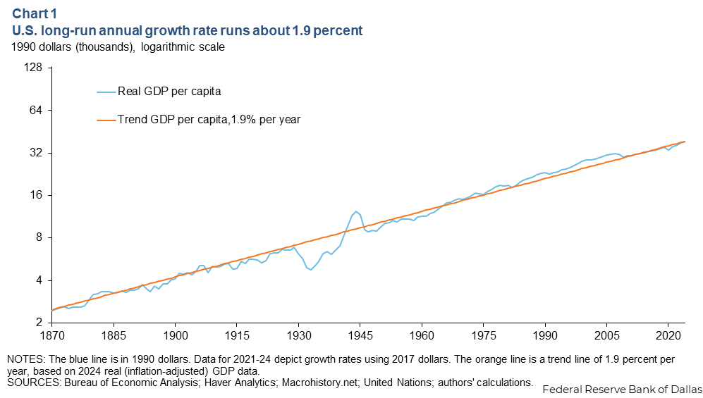
That is a remarkably steady rate of improvement in living standards, especially when one considers the shocks that the U.S. economy experienced over this 150-year period: World War I, the Spanish flu, the Great Depression, World War II, the Great Inflation, the Global Financial Crisis and COVID-19.

There were also many major technological advances such as electrification, the rise of the automobile and the jet engine, biotechnology and the information technology revolution. Moreover, this long-run stability of per-capita GDP growth seems to have been unique to the U.S.

An accounting breakdown of GDP per capita

GDP per capita can increase for many different reasons. To better understand how the increase in living standards can remain so constant over such a long period, we can break down GDP per capita into the following identity:

This is just one of many ways of decomposing changes in living standards over time. Note that a “worker” is someone currently employed, the “labor force” is everyone who is employed and/or actively searching for employment and the “working-age population” is the total population in the defined age range regarded as typically able to work (usually those 15-64 years old).

Higher GDP per capita can occur as a result of increases in any of the terms in this expression: increased labor productivity (more GDP per hour worked), a longer work week (more hours per worker), a higher employment rate, increased labor force participation or a greater share of the population of working age.

However, all but one of the terms in this expression are subject to hard constraints. There is a limit to how many hours a worker can work each week or year; there is also a limit to the share of the labor force that can be employed (100 percent at the maximum, but in reality, a lot less); the labor force participation rate also has a well-defined upper limit (100 percent, but again in reality a lot less). And finally, there is a limit to the share of the population that can be of working age. The only term in this expression that can in principle grow without limit is the labor productivity term.[2]

Exploring this breakdown of growth, GDP per capita can help identify the biggest contributors to changes in living standards on a year-to-year basis and over longer periods of time. Chart 2 plots this decomposition for the post-World War II period.

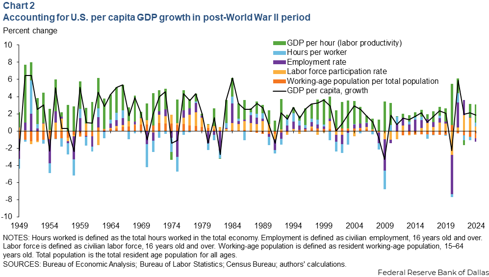
On a year-by-year basis, the various elements of our simple decomposition play a greater or lesser role in improving living standards. In some years, hours per worker make a positive contribution, while in other years they make a negative contribution. Likewise, in some years growth in the share of the population of working age is a drag on living standards, while in other years it acts as a tailwind.

However, a careful examination of the chart shows that the green bar that represents productivity growth is almost always the largest contributor to changes in GDP per capita each year. This is the sense in which productivity growth is central to improvements in living standards over time.

Productivity dominates living standards in all eras

To better see the most significant trends over time, it is helpful to look at a breakdown of GDP per capita over longer time periods (Chart 3).

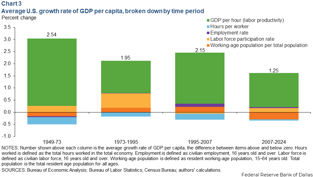
The period from 1949 to 1973 was one of rapid productivity growth. Living standards increased at an average annual rate just above 2.5 percent. That era of rapid productivity growth came to an end around 1973 for reasons that are not fully understood. (The slowdown in productivity growth was not limited to the U.S. but occurred in all advanced economies at around the same time.)

The era of low productivity growth lasted from 1973 to about 1995. This was the period when computer use became more widespread, and MIT economist Robert Solow famously quipped, “You can see the computer age everywhere but in the productivity statistics.”

Computers finally started showing up in the productivity statistics around 1995, and productivity growth picked up again. This period of faster productivity growth lasted for a bit more than a decade, until around the onset of the Global Financial Crisis in 2007. Since 2007, productivity growth has been relatively modest (more akin to what occurred in the 1973–95 period), although there are some signs that it may have begun to pick up in recent years.

Comparing these four eras, there is no trend in the employment rate (and therefore no trend in the unemployment rate). The purple bar remains small and insignificant in all eras, meaning it does not contribute meaningfully to living standards. In addition, hours per worker declined in all four eras as the workweek shortened and vacation days increased.

Looking at the components that shifted significantly between these four eras, the working-age population as a share of the total population was a drag in living standards in the immediate postwar period. The baby boom in the 1940s and 1950s represented a time when the birth rate spiked in the U.S. (Chart 4). This initially caused the contribution of the working-age population as a share of the total population (Chart 3, orange bar) to be a drag on living standards during the 1949–73 period, as the total population grew, increasing the share of the population that was not (yet) of working age.

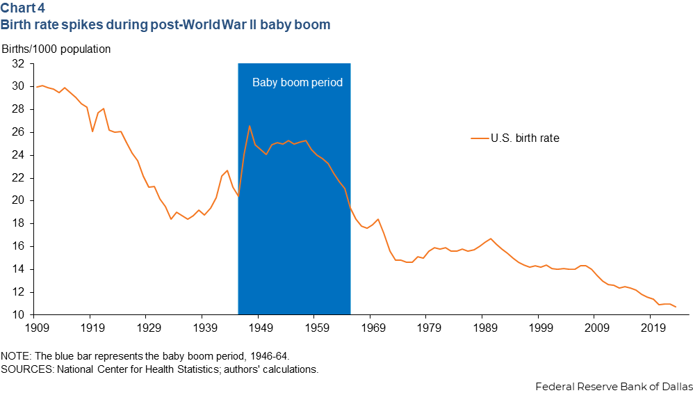
Eventually, of course, the baby boomers came of age, causing the contribution of the working-age population as a share of the total population to turn positive in the 1973–95 and 1995–2007 eras. The contribution of this component once again shifted to negative after 2007, as the boomers retired.

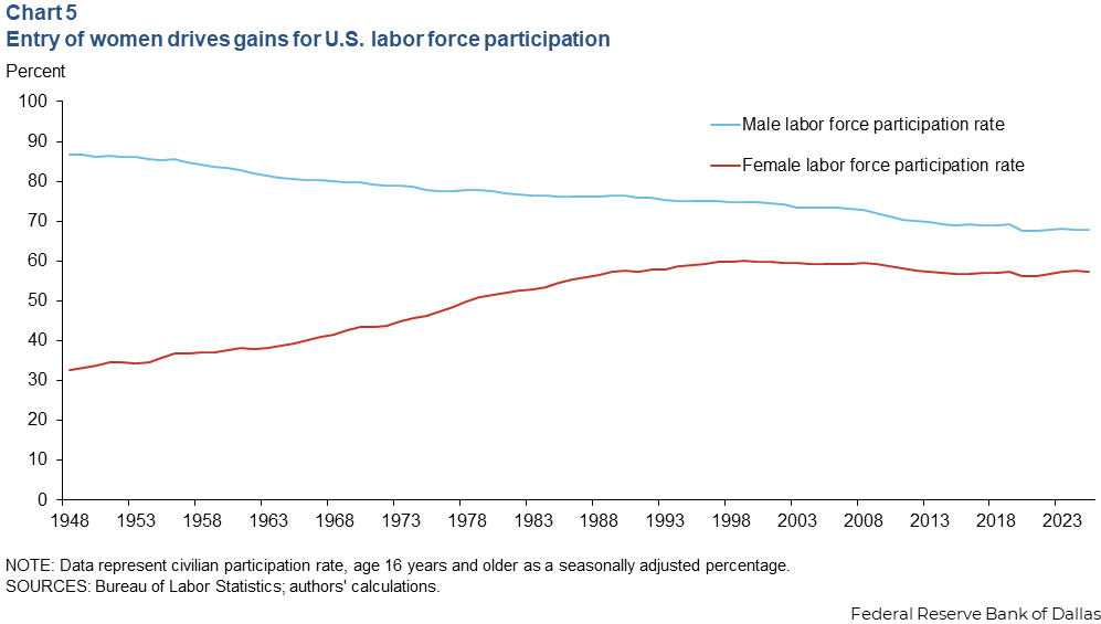
Another example of impact on living standards is a societal shift that began around the 1950s. In Chart 3, the positive light orange bars in 1949–95, and even more prominently in 1973–95, show growth in the labor force participation rate, largely due to the entry of more women into the labor force, which more than offset a decline in male labor force participation over the same period (at least through the early 1990s) (Chart 5).

The consistent positive for all eras is the large green bar in Chart 3, which represents labor productivity. No matter what, labor productivity growth is always positive over long periods of time and is always the largest contributor to higher living standards over time.

Historical data also indicate productivity growth’s importance

This is true not just in the postwar period, but also during the pre-World War II era and through the early 1950s. Due to data limitations, we simplified our accounting identity as follows for the first half of the 20th century:

Chart 6 plots the decomposition on an annual basis. In contrast to what we saw in the post-war data, the pre-war data show much more volatility in the growth of living standards. This period was dominated by two world wars and the Great Depression.

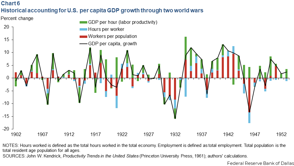
To better break down the historical data, we create averages from 1902–29 (before the Great Depression), 1929–41 (the Great Depression), 1941–46 (World War II) and 1946–53 (the end of the historical data) (Chart 7).

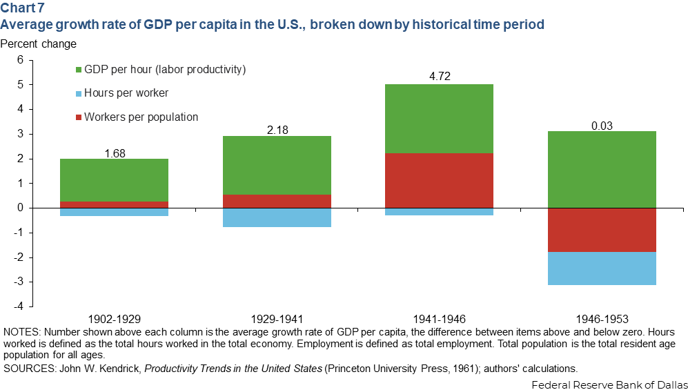
The Great Depression was the greatest economic crisis the U.S. has experienced. Unemployment soared to nearly one quarter of the labor force in 1933. Yet the subsequent recovery was strong enough that by 1941 per capita living standards had grown by an annual average rate of more than 2 percent relative to where they were in 1929.

Real GDP fell 29 percent from 1929 to 1933; the unemployment rate peaked at 26 percent in 1933. Consumer prices, as measured by the deflator for personal consumption expenditures, fell by more than 27 percent between 1929 and 1933. However, in the latter half of the 1930s, productivity peaked and unemployment fell. Thus, during 1929–41, the effects balanced out to relatively neutral growth.

World War II affects this breakdown, too. In the early 1940s, more people entered the workforce—women taking up jobs that men left when going to war—increasing workers per population since the overall population did not change significantly. This accounts for the large brown bar in Chart 7 in 1941–46.

From 1946 to 1953, living standards stagnated: Robust labor productivity growth was barely enough to offset a decline in the employment rate and a reduction in the average hours worked.

Again, in all eras productivity anchored the almost 2 percent growth rate in living standards. The green bar continued to rise, even during wars and crises.

Productivity promotes growth in living standards

Over long periods of time, increases in labor productivity are by far the most important determinants of higher living standards. The ability for productivity to grow limitlessly has allowed living standards to increase at a constant rate over time, no matter what else was going on in the country.

Demonstrating that rising productivity has catalyzed living standards for more than a century reinforces our previous claim that AI may raise living standards over time. In fact, any technology or innovation that increases productivity promotes growth in living standards.

Notes

1. This fact was first documented in Charles I. Jones, “The Facts of Economic Growth,” in Handbook of Macroeconomics Volume 2A, ed. John B. Taylor and Harald Uhlig (Elsevier, 2016). Earlier research by Nancy Stokey and Sergio Rebelo in “The Growth Effects of Flat-Rate Taxes,” Journal of Political Economy, vol. 103, no. 3 (1995): 519–50, also documented the remarkable constancy of the trend growth rate of the U.S. economy over long periods of time despite significant variation in tax rates. This work buttressed an earlier finding by Robert E. Lucas, Jr., “Supply-Side Economics: An Analytical Review,” Oxford Economic Papers, vol. 42, no. 2 (1990): 293-316, in that eliminating the taxation of capital income and replacing the lost revenue by raising the tax rate on labor income so as to keep overall government revenue constant would have a trivial effect of the U.S. growth rate.
2. We focus on the concept of labor productivity. There is a more comprehensive measure of productivity known as total factor productivity (TFP), which takes into account the fact that labor is not the only factor of production, which also includes capital. Labor productivity growth can occur as a result of more capital being available for each worker to work with (an increase in the capital labor ratio) or as a result of TFP growth. Arguably, there are limits to how much capital can be made available to each worker (capital accumulation of necessity requires forgoing consumption), so at the end of the day the potential for labor productivity to grow without limit is ultimately due to the ability of TFP to grow without limit. TFP is more difficult to measure than labor productivity, as it typically requires some assumptions about the way in which capital and labor are combined to produce final output. It also requires accurate measurement of the service flow of the capital stock: A given stock of capital may be utilized more or less intensively depending on where an economy is in the business cycle. These measurement challenges have grown in recent years with the increased importance of intangible capital. For a discussion of some of these issues, see for example Nicolas Crouzet and Janice Eberly, “Intangibles, markups, and the measurement of productivity growth,” Journal of Monetary Economics, vol. 124 (November 2021): S92–S109.